Lesson 4: Set Up the Spreadsheet

A paper transaction register is part of the past, but its purpose never will be. With a spreadsheet, manual computing is no longer needed. And forget about sloppy handwriting. Typed entries are the way to go.

In order to use the data collected in Lesson 3: Get Ready, follow the steps below to get set up.

1. Select a spreadsheet application
2. Log into Google
3. Set up the spreadsheet
4. Add balance formula and duplicate
5. Format the cells

Select a Spreadsheet Application

There are multiple software applications to choose from. For example, Microsoft Excel and Google Sheets. Given Google Sheets is free, this lesson will assume a Google solution. However, the steps to set up the spreadsheet can be used in Excel.

Log Into Google

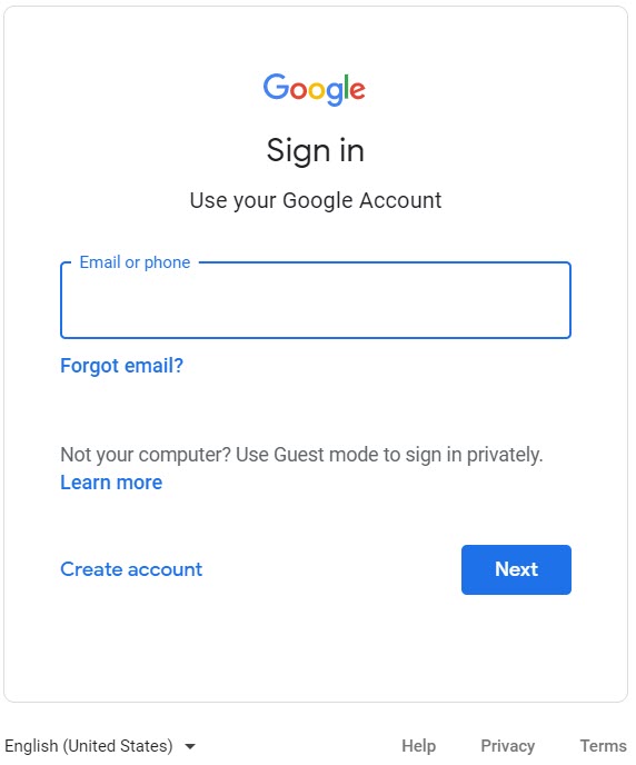
If you have an account, login. In fact, it’s likely that you already are. If you aren’t sure, go to https://www.google.com/. Do you see the Sign In Button? If not, you are logged in.

You if see the button, click it and log in. If you don’t have an account, create one with the following instructions. Don’t worry, you don’t need a Google email to create a Google account. I didn’t.

1. Go to https://accounts.google.com/
2. Click on Create account and follow the steps that Google asks you to complete.

Set Up the Spreadsheet

Now that you are logged in, go to your Google drive and start setting up your spreadsheet.

1. Go to https://drive.google.com/ 
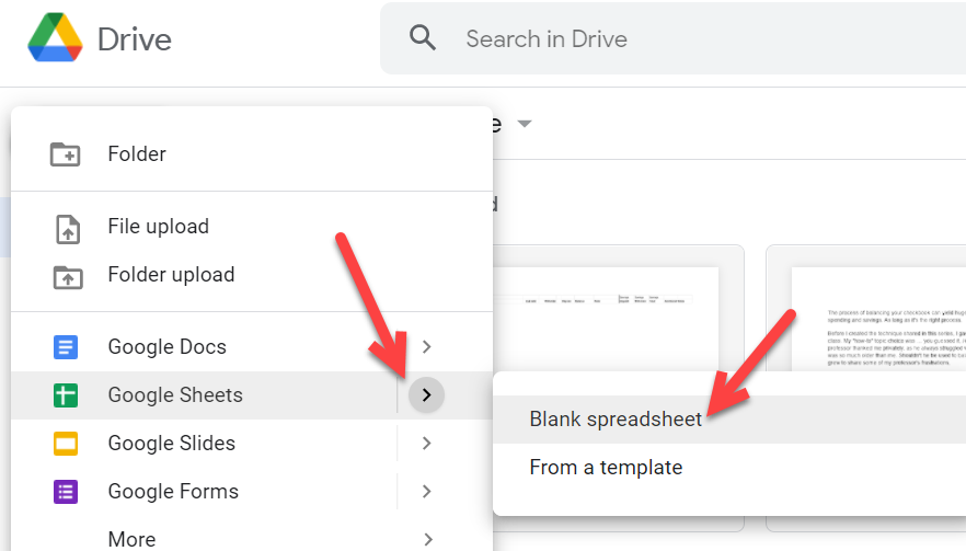
2. Click on the New button.

3. Select Google Sheets then Blank spreadsheet.

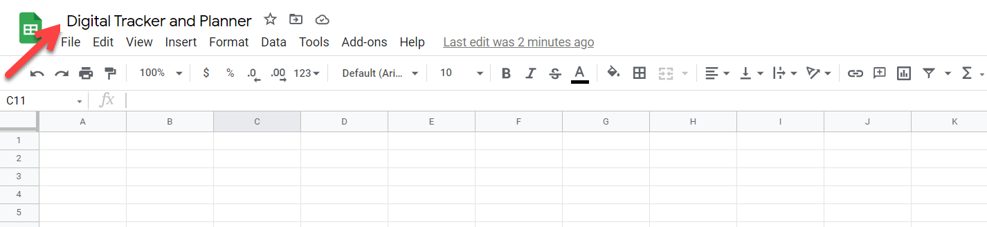
4. Observe the blank sheet. An Excel spreadsheet will be similar, if you choose that option.

5. Enter a sheet name: Digital Tracker and Planner.

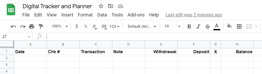
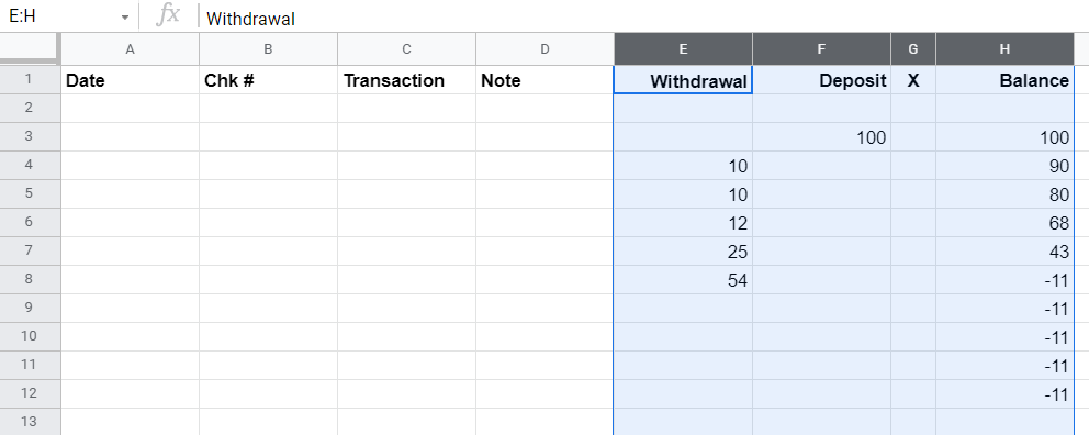
6. Enter column headers: Date, Chk # (i.e., check number), Transaction, Note, Withdrawal, Deposit, X, Balance.

Add the Balance Calculations

There are two simple calculations performed when managing your checking account balance:

• Balance minus check written = new balance.
• Balance plus deposit = new balance

The power of the spreadsheet allows you to perform both calculations at the same time. The formula for row 3 under the balance column is =H2+F3-E3, where the balance cell equals the balance from the cell above plus the deposit minus the withdrawal. You can enter it once at the top and duplicate it down the balance column, per the instructions below. 

1. Enter the formula in the third cell under the balance column: =H2+F3-E3. If you are familiar with building formulas by clicking on cells, feel free to do so.

2. Next, duplicate the formula by clicking on the formula cell. Hold down the shift key and arrow down to highlight cells below. 

3. Click Ctrl+D on a PC or Command+D on Mac to duplicate the formula. Ultimately, you will duplicate the formula to the end of the 12 months of planned commitments, but you will do that later.
4. To see what the formula in action, enter some numbers in the withdrawal and deposit columns. See the balance change from row to row.

Format the Cells

The example numbers in figure 11 generated a negative balance. The little minus sign in front of the negative numbers doesn’t stand out. And, not all entries will be even dollars. Let’s apply a format to the three number columns. 

1. Highlight the money columns E through H. Don’t worry about the G column not being a number column. It will still accept an X for each transaction checked against the bank.

2. Click on the 123 dropdown in the editor bar and select Custom number format.

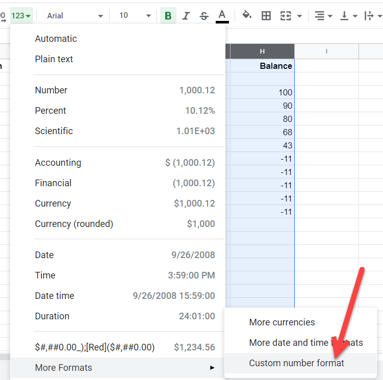
3. Select the format $#,##0.00_);[Red]($#,##0.00).

4. Observe the results.

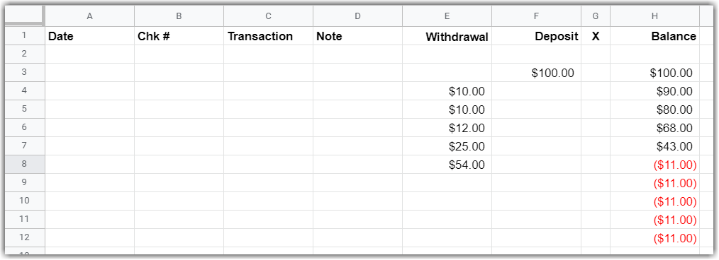
• The numbers now look like dollars.
• The negative balance is now in red, much easier to notice. An important feature.

Imagine the numbers you entered were real and that they were predictions of future commitments and balance. The scenario above suggests that a $54.00 commitment will not be doable unless additional money is deposited or other commitments are postponed.

Next Lesson …

The next lesson depends on when you get paid. Choose the lesson that best applies to your situation. Lesson 5d assumes you have completed either 5a, 5b, or 5c.

• Lesson 5a: Single Monthly Paycheck Plan
• Lesson 5b: Twice a Month Paycheck Plan
• Lesson 5c: Every Two Weeks Paycheck Plan
• Lesson 5d: Front Loaded Paycheck Plan